Introduction to Continuous
Markov Chains & Queueing Theory
in Healthcare Supply Chains

Udeshi Salgado
Data Lab for Social Good,
Cardiff University, UK
2025-05-22

Assumptions

• You should be familiar with basic probability and random variables.
• You are expected to be comfortable with R (or Python) for basic simulation and matrix operations.
• This is not a theory-heavy workshop—we will use simple examples to build intuition, not derive theorems.

What We Will Cover

• Key concepts and steady-state analysis of Continuous-Time Markov Chains (CTMCs)
  
• Modeling a vaccine observation room using CTMCs
• Introduction to Queueing Theory
• Introduction to M/M/1 queueing systems and performance metrics

What We Will Not Cover

• Theoretical proofs (e.g., Chapman-Kolmogorov, Little’s Law)
  
• Networks of queues
• Multiclass queues and priority scheduling
  
• Non-stationary arrivals and general service times
• Non-exponential queues
• Time-dependent queueing models

Materials

• You can find the workshop materials at here.
• Note: These materials are based on my learnings at NATCOR Taught Course Centre: Stochastic Modelling Course

Outline

1. Recap
2. Continuous Time Markov Chains (CTMC)
3. Lab Activity: Part 1 – CTMC (Vaccine Observation Room)
4. Queueing Theory
5. Lab Activity: Part 2 – Queueing Theory (Check-In Desk)

Recap: Quiz Time!

Recap: Discrete-Time Markov Chain (DTMC) Assumptions

• The system is always in exactly one state at any given time step.
• The next state depends only on the current state, not on the past (Markov property).
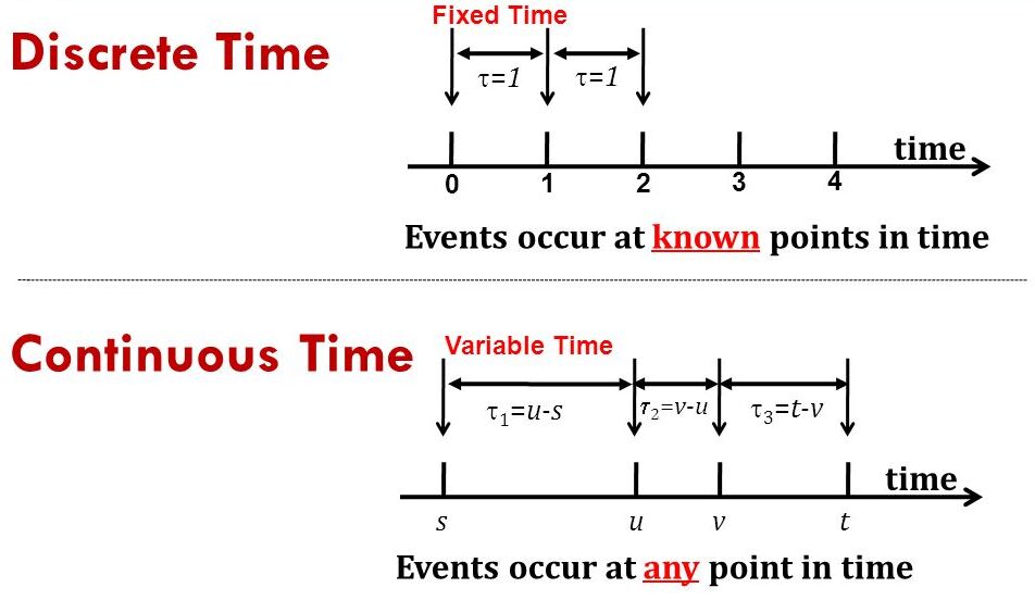
• Transitions happen at fixed, regular time steps.
• Transition probabilities stay the same over time.

Recap: State Space and Parameter Space

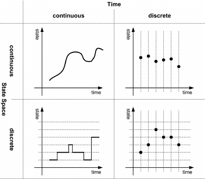
Recap: Discrete MC Vs Continuous MC

Outline

1. Recap
2. Continuous Time Markov Chains
3. Lab Activity: Part 1 – CTMC (Vaccine Observation Room)
4. Queueing Theory
5. Lab Activity: Part 2 – Queueing Theory (Check-In Desk)

Continuous Time Markov Chains (CTMC)

• In a continuous-time Markov chain (CTMC), the system state can change at any point on the continuous time axis.

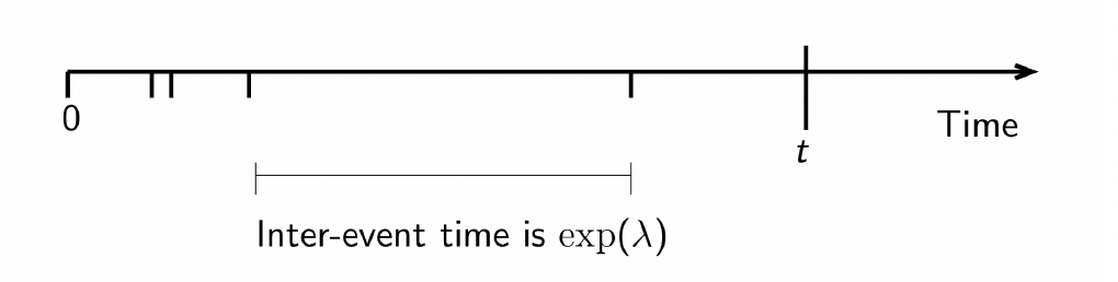
Exponential Timing in CTMCs

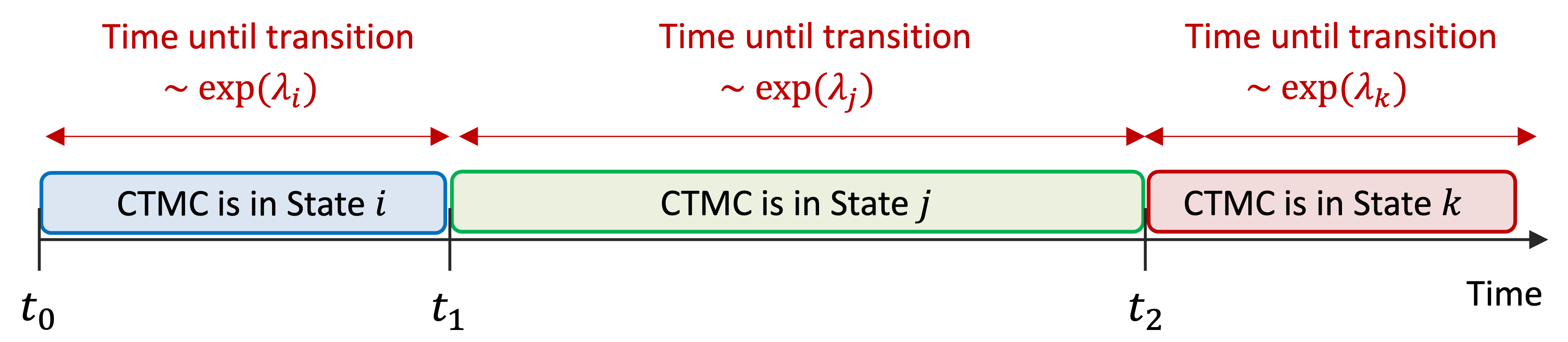
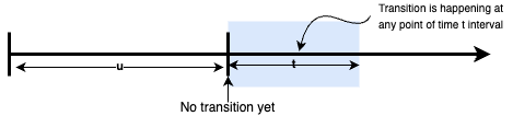
• Assumption: In a Continuous-Time Markov Chain (CTMC), the time until the next state transition is modeled as a random variable
  \[ T \sim \text{Exponential}(\lambda) \]
  where:
  • \(T\) = time until next transition
    
  • \(\lambda > 0\) = transition rate (higher \(\lambda\) → faster transitions)

Exponential Timing in CTMCs Cont.

• The memoryless property of the exponential distribution:
  \[ \Pr(T > t + u \mid T > u) = \Pr(T > t) \quad \text{for all } t, u > 0 \]

• Interpretation: Time already spent in the current state does not influence the probability of future transitions.

• This is consistent with the Markov property: The future depends only on the current state, not the past.

Key Concepts: Stochastic Process, Time & State Spaces

• A stochastic process is a collection of random variables \(\{X(t)\}\) indexed by time \(t\).

• The parameter space defines the set of time points:

  • For continuous-time processes: \(t \in [0, \infty)\).

• The state space \(S\) is the set of all possible values \(X(t)\) can take:

  • Typically finite or countably infinite, e.g., \(S = \{0, 1, 2, \dots\}\).

• \(X(t)\) represents the state of the system at time \(t\).

CTMCs: Definition

A continuous-time Markov chain (CTMC) is a stochastic process:

\[ \{X(t) \mid t \geq 0\} \]

where:

• \(X(t)\) is a random variable representing the system’s state at time \(t\).
• \(t\) belongs to the parameter space \([0, \infty)\).
• The values of \(X(t)\) come from a state space \(S\), usually finite or countable.

CTMCs: Definition Cont.

The process satisfies the Markov property:

\[ \Pr(A \mid X(t),\, 0 \leq t \leq T) = \Pr(A \mid X(T)) \]

where:

• \(A\) is any future event.
• The future depends only on the current state \(X(T)\), not on the history.

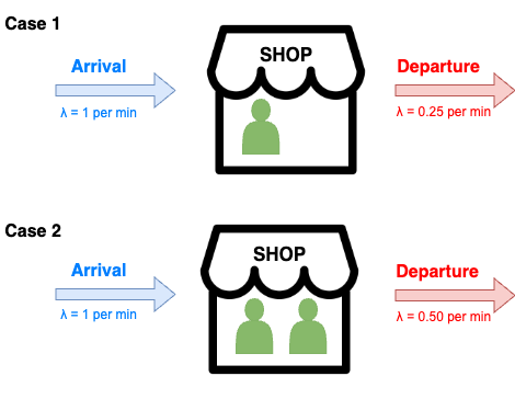
CTMC Example: Managing a Tiny Shop’s Flow

Imagine a small neighborhood pharmacy with space for maximum of two customers at a time. As the shop owner, you’re analyzing foot traffic to optimize customer experience without overcrowding or turning people away.

CTMC Example: Managing a Tiny Shop’s Flow Cont.

• Arrivals follow an exponential distribution with λ = 1 per minute
• Departures depend on how many customers are in the shop:
  • 1 customer → exponential(λ = 0.25)
  • 2 customers → exponential(λ = 0.5)
• If a new customer arrives:
  • And there are 0 or 1 customers, they enter the shop
  • If 2 customers are already inside, they leave without entering (no queueing!)

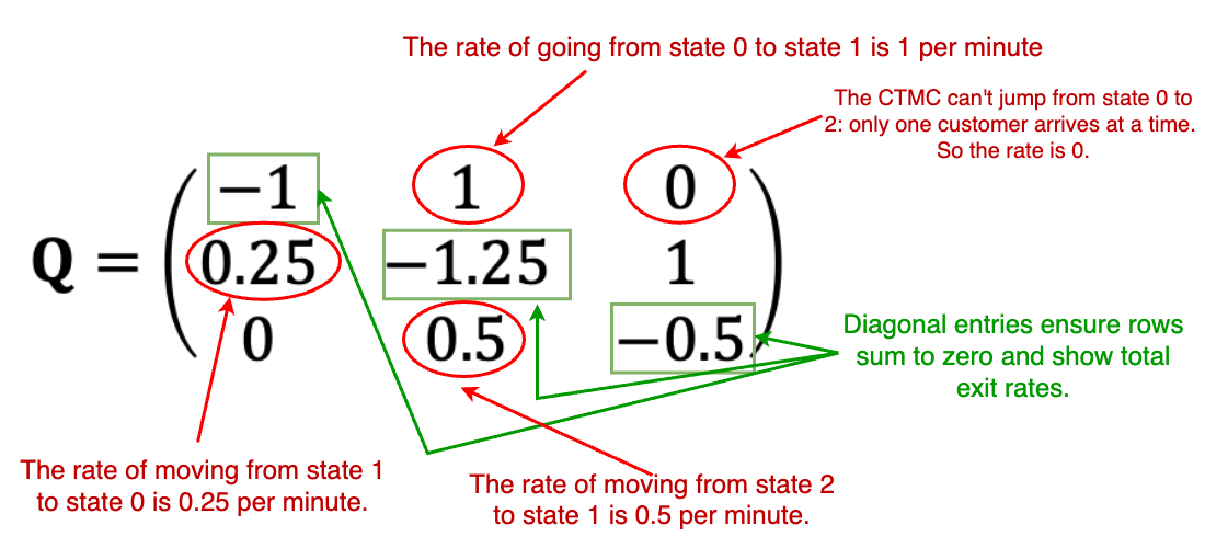
CTMC Example: Transition Rate Diagram

• We can model this scenario as a Continuous-Time Markov Chain (CTMC), where the state represents the number of customers in the shop.
• Thus, the possible states are: 0, 1, and 2.
• We can visualize the transition rates between these states:

Time Until Next Transition

Let \(T_i\) be the time until the next transition from state \(i \in \{0, 1, 2\}\)

• \(T_0 \sim \text{Exp}(1)\) (arrival triggers transition)

• \(T_2 \sim \text{Exp}(0.5)\) (departure triggers transition)

• \(T_1 = \min(A, D)\), where:

  • \(A \sim \text{Exp}(1)\) (a new customer arrives)
  • \(D \sim \text{Exp}(0.25)\) (a customer leaves the shop)

Exponential Minimum Property

Suppose \(T_1\), \(T_2\) are independent and \[ T_1 \sim \text{Exp}(\lambda_1),\quad T_2 \sim \text{Exp}(\lambda_2) \]

Then:
\[ \min(T_1, T_2) \sim \text{Exp}(\lambda_1 + \lambda_2) \]

Exponential Minimum Property Cont.

Application to our example:

• For state 1:
  \[ T_1 = \min(A, D); \quad A \sim \text{Exp}(1),\ D \sim \text{Exp}(0.25) \]
• So:
  \[ T_1 \sim \text{Exp}(1 + 0.25) = \text{Exp}(1.25) \]

Generator Matrix for a CTMC

The generator matrix (Q) summarizes the transition rates between states in a CTMC.

• Each element \(q_{ij}\) gives the rate of moving from state \(i\) to state \(j\)
• Diagonal elements are negative and equal to the negative of the row sum
• Non-diagonal elements are \(\geq 0\) and indicate direct transitions

Interpreting Key Entries in Generator Matrix

Steady-State Probabilities

Steady-state probabilities represent the long-run behavior of the system.
They tell us:

• The proportion of time the CTMC spends in each state in the long run.
• The limiting probability that the system is in a given state after a long time.

To find them, we solve: \[ \boldsymbol{\pi} \mathbf{Q} = \mathbf{0}, \quad \text{with} \quad \sum \pi_i = 1 \]

Where: \(Q\) is the generator matrix of the CTMC, \(\boldsymbol{\pi}\) is a row vector of steady-state probabilities.

Solving the System

From:

\[ \begin{aligned} &-\pi_0 + 0.25\pi_1 = 0 \\ &\pi_0 - 1.25\pi_1 + 0.5\pi_2 = 0 \\ &\pi_1 - 0.5\pi_2 = 0 \\ &\pi_0 + \pi_1 + \pi_2 = 1 \end{aligned} \]

Thus: \[ \pi_0 = \frac{1}{13},\quad \pi_1 = \frac{4}{13},\quad \pi_2 = \frac{8}{13} \]

Long-run Average Number of Customers

We calculate:

\[ 0 \cdot \frac{1}{13} + 1 \cdot \frac{4}{13} + 2 \cdot \frac{8}{13} = \frac{20}{13} \approx 1.54 \]

This is the expected number of customers in the shop in the long run.

Summary of CTMCs

• Transition times are exponentially distributed.
• The generator matrix \(\mathbf{Q}\) defines transition rates.
• Steady-state \(\boldsymbol{\pi}\) solves:
  \[ \boldsymbol{\pi} \mathbf{Q} = 0, \quad \sum \pi_i = 1 \]
• \(\pi_i\) gives long-run proportions of time spent in each state.

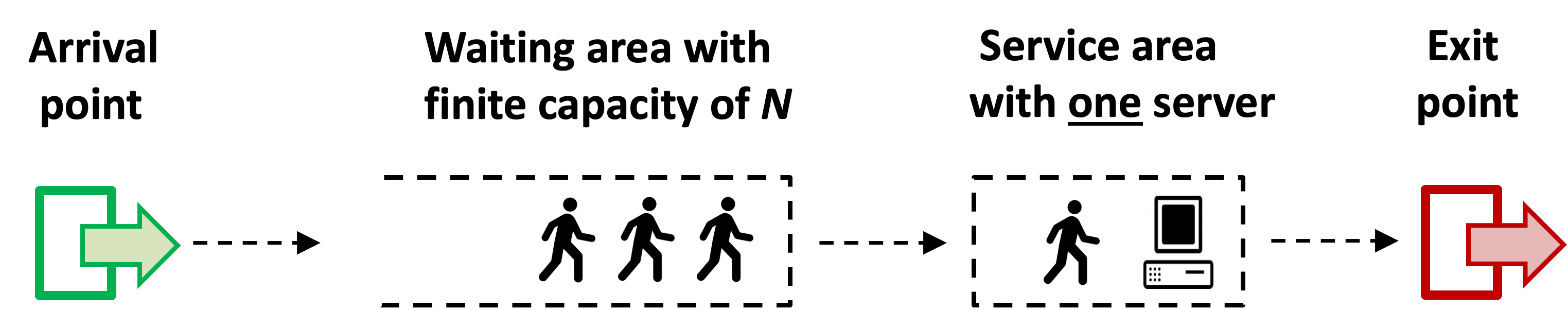
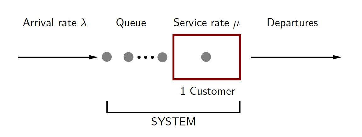
Queueing Systems as CTMCs

A queueing system (e.g., customer service desk, call center, clinic) can often be modeled as a continuous-time Markov chain, under assumptions like:

• Exponentially-distributed inter-arrival times
• Exponentially-distributed service times
• Finite waiting area, single server, and one-at-a-time processing

Outline

1. Recap
2. Continuous Time Markov Chains (CTMC)
3. Lab Activity: Part 1 – CTMC (Vaccine Observation Room)
4. Queueing Theory
5. Lab Activity: Part 2 – Queueing Theory (Check-In Desk)

Lab Activity: Part 1 – CTMC (Vaccine Observation Room)

In this section, you’ll model an observation room where recently vaccinated patients are monitored for adverse events. The room has limited capacity (e.g., 2 beds).

We will use a Continuous-Time Markov Chain (CTMC) to:

• Construct the generator matrix (\(Q\))
• Write and solve the steady-state equations
• Interpret the long-run distribution across states

Make sure you load the required R packages: Matrix, expm

Outline

1. Recap
2. Continuous Time Markov Chains (CTMC)
3. Lab Activity: Part 1 – CTMC (Vaccine Observation Room)
4. Queueing Theory
5. Lab Activity: Part 2 – Queueing Theory (Check-In Desk)

Queueing Theory

Welcome to Queueing Theory!
We’ll explore how to model and analyze systems where “waiting” happens — like hospitals, call centers, and shops.

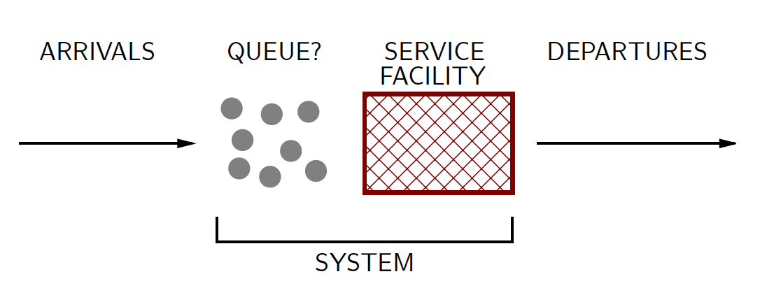
What is a Queueing System?

A system with:

• Arrivals (e.g., customers, calls)
• A queue (optional)
• Service process (1 or more servers)
• Departures

Real-World Applications

• ATM and supermarket checkout lines
• Call centers and helpdesks
• Hospital patient flow
• Computer servers and networks

Kendall’s Standard Notation

Queueing systems are described using: A/B/S/d/e

• A – Arrival distribution (e.g., M = Exponential)
• B – Service distribution (e.g., M, D = Deterministic, G = General)
• S – Number of servers
• d – System capacity (buffer size)
• e – Queue discipline (e.g., FIFO, LIFO)

Example: M/M/2/5/FIFO

→ Exponential arrivals, exponential service, 2 servers,
→ Max 5 customers in system, served in order of arrival

Poisson Process

• Many queueing systems assume Poisson arrivals, a key foundation for M/M/1 and related models.
• This process is simple but powerful and forms the basis for most queueing models.

Definition:
A Poisson process with rate \(\lambda\) models random arrivals over time, where:

Poisson Process Cont.

• The number of arrivals in time \(t\) follows:
  \[ P(N(t) = k) = \frac{(\lambda t)^k e^{-\lambda t}}{k!} \]
• Interarrival times are exponentially distributed:
  \[ T \sim \text{Exp}(\lambda) \]
• Memoryless: the probability of arrival doesn’t depend on the past

The M/M/1 Queue

• A single-server queue with:
  • Exponential interarrival times (rate \(\lambda\))
  • Exponential service times (rate \(\mu\))
• The number of customers in the system defines the state
• The queue has infinite capacity

The M/M/1 Queue Cont.

Traffic intensity: How busy the system is? \[ \rho = \frac{\lambda}{\mu} \]

• If \(\rho < 1\), the system reaches a steady-state
• If \(\rho \geq 1\), the queue grows indefinitely
• \(\lambda\) = arrival rate, \(\mu\) = service rate

💡 Think of \(\rho\) as the load on the server.
If arrivals outpace service, the system can’t cope.

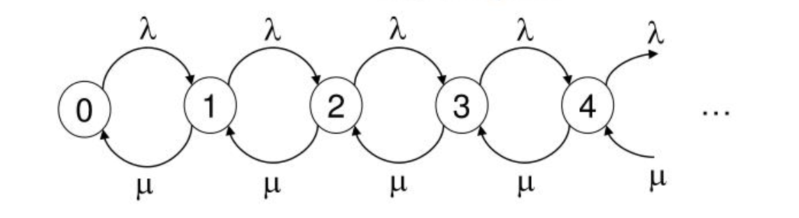
M/M/1 as a CTMC

• The M/M/1 queue can be modeled as a Continuous-Time Markov Chain (CTMC).
• States represent the number of customers in the system: 0, 1, 2, …
• The process is a birth–death process:
  • Births (arrivals) occur at rate \(\lambda\)
  • Deaths (departures) occur at rate \(\mu\)

M/M/1 as a CTMC Cont.

Generator matrix (Q):

\[ \mathbf{Q} = \begin{pmatrix} -\lambda & \lambda & 0 & 0 & \cdots \\ \mu & -(\lambda + \mu) & \lambda & 0 & \cdots \\ 0 & \mu & -(\lambda + \mu) & \lambda & \cdots \\ \vdots & \vdots & \ddots & \ddots & \ddots \end{pmatrix} \]

• This structure defines the dynamics of the queue over time.

M/M/1: Stationary Distribution & Performance

Assume the system reaches steady state (\(\rho < 1\)), with probabilities \(\{p_n,\ n \geq 0\}\).

These come from solving the balance equations of the CTMC:

State 0 balance:

\[ \lambda p_0 = \mu p_1 \]

For \(n \geq 1\):

\[ (\lambda + \mu)p_n = \lambda p_{n-1} + \mu p_{n+1} \]

Solving recursively gives:

\[ p_n = \rho^n p_0 \quad \text{where} \quad \rho = \frac{\lambda}{\mu} \]

Then apply the normalization condition:

\[ \sum_{n=0}^\infty p_n = 1 \quad \Rightarrow \quad p_0 = 1 - \rho \]

So we get:

• Probability the system is empty:
  \[p_0 = 1 - \rho\]

• Probability the server is busy:
  \[1 - p_0 = \rho\]

• Probability of \(n\) customers in the system:
  \[p_n = \rho^n (1 - \rho)\]

🧠 These describe the stationary distribution of the M/M/1 queue.

M/M/1: Mean Number in System (\(L\))

Expected number of customers in the system:

\[ L = \sum_{n=0}^{\infty} n p_n = \sum_{n=0}^{\infty} n \rho^n (1 - \rho) = \rho \sum_{n=1}^{\infty} n \rho^{n-1} (1 - \rho) = \frac{\rho}{1 - \rho} \]

• This is one of the key performance metrics in queueing analysis.
• \(L\) increases sharply as \(\rho \to 1\), showing how queues explode near capacity.

💡 Use this to inform decisions on service rates (\(\mu\)) to keep queues manageable.

Performance Measures in Queueing

Four key summary performance measures:

• \(L\): Mean number of customers in the system
• \(L_q\): Mean number of customers in the queue
• \(W\): Mean time a customer spends in the system
• \(W_q\): Mean time a customer spends waiting in the queue

Little’s Law

A fundamental relationship linking arrival rate, waiting time, and number in the system.

Mean number of customers in the system:

\[ L = \lambda W \qquad \text{($\lambda$ = arrival rate, $W$ = mean time in system)} \]

Also:

\[ L = L_q + \frac{\lambda}{\mu} \qquad \text{(total in system = queue + in service)} \]

Mean waiting time:

\[ W = W_q + \frac{1}{\mu} \qquad \text{($W_q$ = time in queue, $\frac{1}{\mu}$ = service time)} \]

Mean number of customers in the queue:

\[ L_q = \lambda W_q \qquad \text{($\lambda$ = arrival rate, $W_q$ = mean time in queue)} \]

M/M/1 Queue: Performance Formulas

Using \(\rho = \frac{\lambda}{\mu}\) and Little’s Law:

• Mean number in the system: \[ L = \frac{\rho}{1 - \rho} \]

• Mean number in queue: \[ L_q = \frac{\rho^2}{1 - \rho} \]

M/M/1 Queue: Performance Formulas Cont.

• Mean time in the system: \[ W = \frac{1}{\mu(1 - \rho)} \]

• Mean waiting time in queue: \[ W_q = \frac{\rho}{\mu(1 - \rho)} \]

Comparing M/M/1, M/M/s, and M/M/s/b

Feature	M/M/1	M/M/s	M/M/s/b
Servers	1	\(s\)	\(s\)
System Capacity	Infinite	Infinite	\(b\) (finite)
Arrival Rate (\(\lambda\))	Poisson	Poisson	Poisson
Service Time	Exponential	Exponential	Exponential
Queue Capacity	Infinite	Infinite	\(b - s\)
Blocking?	No	No	Yes (if system full)
Common Use	Basic single-server queue	Multi-server (e.g., call center)	Limited capacity (e.g., hospital beds)

Let’s Practice: Model Matching

You’ll see 3 real-world situations.
For each one, pick the most suitable queueing model:

• M/M/1
• M/M/s
• M/M/s/b

You’ll have 30 seconds to discuss or decide for each!

Scenario 1

An emergency care unit in a district hospital has five treatment beds. Once all beds are occupied, incoming patients must be transferred to a different facility, as there is no space for waiting or holding.

Which queueing model applies?

• M/M/1
  
• M/M/s
  
• M/M/s/b

Scenario 1 – Answer

M/M/s/b Queueing Model

- Multiple beds = multiple servers
- No waiting space = limited capacity
- Incoming patients are blocked if full

Scenario 2

A mobile vaccination clinic is staffed by a single nurse. Patients from a rural community arrive randomly and are vaccinated one at a time. If the nurse is busy, others wait in line without any restrictions on queue length.

Which model applies?

• M/M/1
  
• M/M/s
  
• M/M/s/b

Scenario 2 – Answer

M/M/1 Queueing Model

• One nurse = one server
  
• Unlimited queue = no blocking
  
• Standard basic queueing setup

Scenario 3

A city hospital’s diagnostic laboratory operates with four technicians. Incoming test samples are processed as soon as a technician is free. If all are busy, samples wait in a queue with no limit.

Which model applies?

• M/M/1
  
• M/M/s
  
• M/M/s/b

Scenario 3 – Answer

M/M/s Queueing Model

• Four technicians = multiple servers
  
• Queue allowed = no blocking
  
• Standard multi-server queue

Outline

1. Recap
2. Continuous Time Markov Chains (CTMC)
3. Lab Activity: Part 1 – CTMC (Vaccine Observation Room)
4. Queueing Theory
5. Lab Activity: Part 2 – Queueing Theory (Check-In Desk)

Lab Activity: Part 2 – Queueing Theory (Check-In Desk)

In this section, you’ll model the check-in desk where patients arrive and wait to be registered by a nurse.

We will use an M/M/1 queue to:

• Calculate traffic intensity (\(\rho = \lambda / \mu\))
• Compute steady-state metrics:
  • Average number in system (\(L\)) and queue (\(L_q\))
  • Waiting times (\(W\), \(W_q\))
• Reflect on how arrival/service rates affect congestion

You’ll be guided with real-world tasks followed by code. Let’s begin!