Forecasting Routine Vaccine Administration Under Uncertainty

A Comparative Evaluation

Udeshi Salgado, Cardiff University, UK
Lead supervisor: Prof. Bahman Rostami-Tabar
Co-supervisors: Dr Thanos E Goltsos, Dr Geraint Palmer, Dr Paul Wang
Data Lab for Social Good, Cardiff University, UK

30 June 2026

Outline

• Background and motivation
• Current practice: the FSP tool
• Data and Methodology
• Results

Outline

• Background and motivation
• Current practice: the FSP tool
• Data and Methodology
• Results

Background

• 1 in 5 children worldwide still lack access to essential vaccines.
• A key operational driver is inefficiency in vaccine supply chains.
• In low and middle-income countries this shows up as:
  • inaccurate demand forecasts
  • inventory decisions made with no measure of uncertainty
  • wastage and stockouts

Vaccines

A vial holds several doses; each dose is what reaches a child. We forecast the doses actually administered.

Vial

Dose

Administered

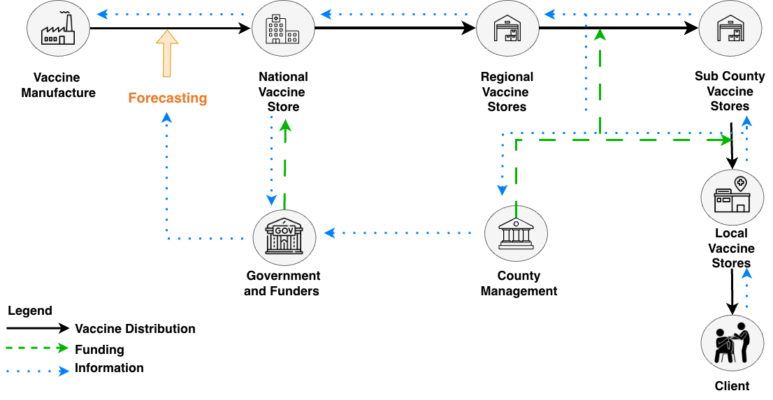
The immunisation supply chain

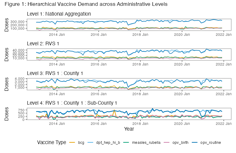
Demand across administrative levels

Outline

• Background and motivation
• Current practice: the FSP tool
• Data and Methodology
• Results

One question, three answers

How many doses to procure next year? FSP4All forecasts consumption (administered doses plus wastage) three ways, then blends them.

Demographic

• Counts the eligible child population
• Coverage target × dose schedule
• \(Q_{\mathrm{dem}} = P \cdot \frac{c}{100} \cdot d\)

Consumption

• Averages the last 12 months of issues into one flat mean
• Projects it forward by assumed growth, even when the data are years old
• \(Q_{\mathrm{cons}} = \bar{C} \cdot 12 \cdot (1+g)^{t} \cdot \frac{100-w_{\mathrm{old}}}{100-w_{\mathrm{new}}} \cdot (1+r)\)

Session

• Built bottom-up from the session plan
• Sessions × average attendance × doses
• \(Q_{\mathrm{sess}} = \sum_{s} n_{s} \cdot \bar{a}_{s} \cdot d\)

Then combine

• \(Q_{\mathrm{FSP}} = \sum_{m} \omega_{m}\, Q_{m}\)
• Weights are decided by the experts in the immunisation supply chain. Default weights are equal

Notation \(P\): target population
\(c\): coverage (%)
\(d\): doses per child
\(\bar{C}\): avg. monthly consumption
\(g\): population growth
\(t\): years from data to plan year
\(r\): planner’s manual % adjustment, e.g. for a campaign
\(w\): wastage (%)
\(n_s\): sessions
\(\bar{a}_s\): attendance
\(\omega_m\): method weights

The data is there, but the method isn’t

Two methods have no inputs; the third ignores the history sitting right beside it.

Session   No data

• No session plans kept
• No attendance records
• The method cannot run

Consumption   No data

• Only administered doses recorded
• No wastage or reporting rates
• Consumption cannot be computed

Demographic   Data, but…

• A fixed estimate, not a forecast
• Needs a rarely-measured wastage rate
• Uncertainty stays hidden

The missed opportunity. FSP4All already holds both the demographic estimate and years of doses-administered history. Yet it only averages them, using simple or expert-assigned weights. No forecasting model is ever fitted to the historical data.

Outline

• Background and motivation
• Current practice: the FSP tool
• Data and Methodology
• Results

Data

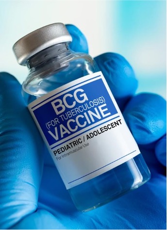
5 vaccines BCG · Pentavalent · Measles-Rubella · OPV birth · OPV routine

306 sub-counties the most granular operational level

1,530 series one per vaccine and sub-county

Monthly, 2013 to 2021 doses administered, calendar-normalised

Demographic and coverage FSP target population · WHO coverage targets

External drivers floods · drought · epidemics · CPI · holidays

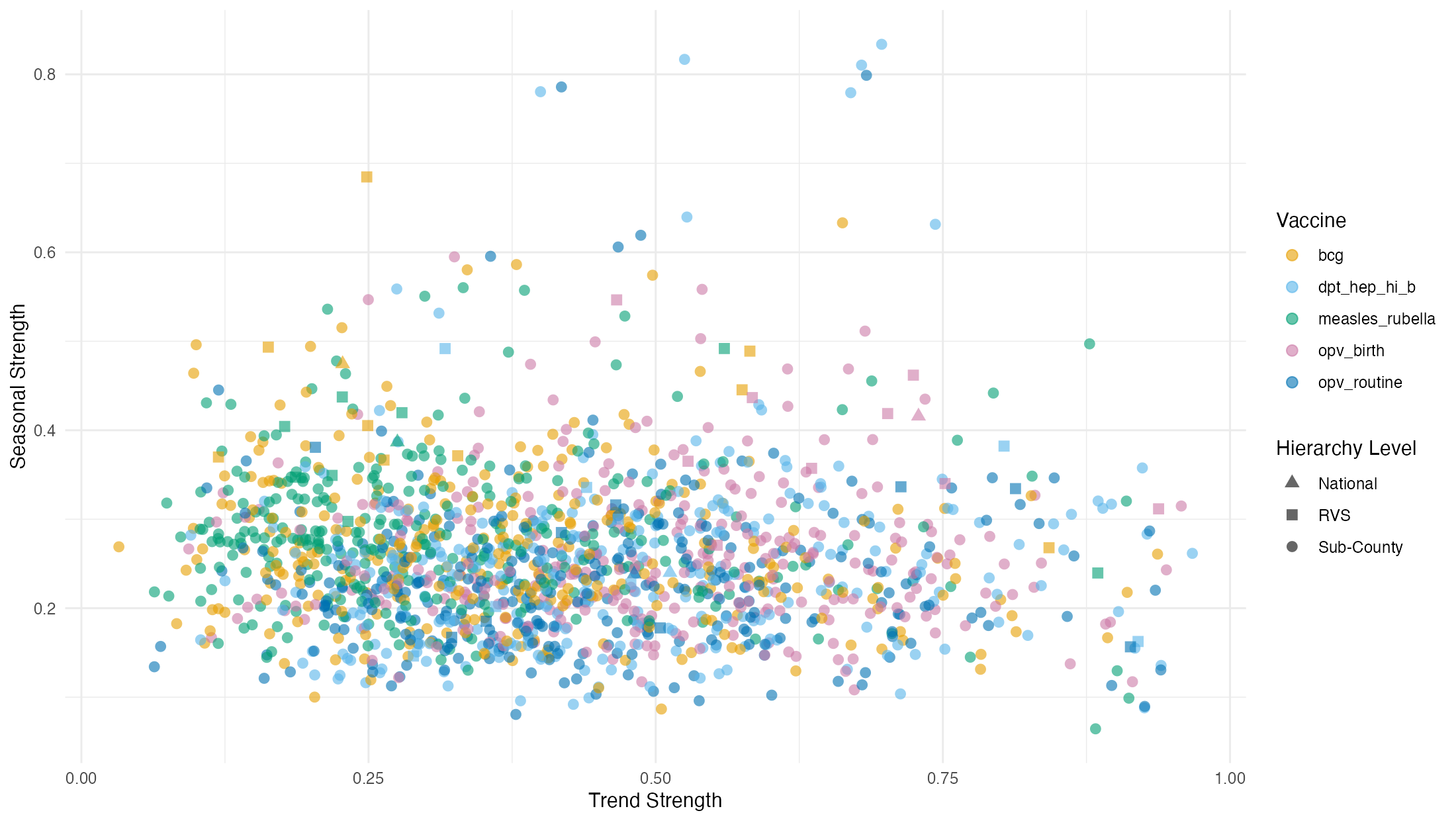
Weak trend and seasonality

Across the 1,530 series, most show low trend strength and weak, inconsistent seasonality. Sub-county series (circles) are the noisiest and least predictable, so historical patterns alone explain only part of demand.

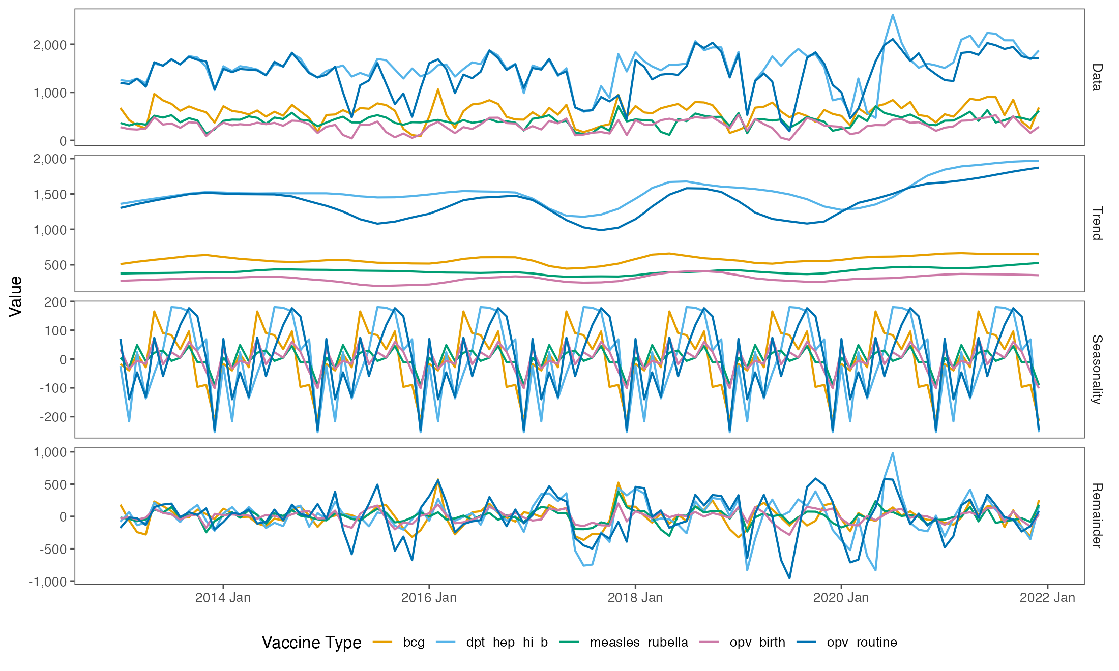
Trend, seasonality and noise

Decomposing the administered series: a smooth local trend and a modest seasonal cycle sit beneath a large, irregular remainder. At the operational level the noise component dominates.

Forecast the history, bound with the plan

We hold administered doses, not consumption. So we forecast administered demand with uncertainty and bound it with the administered demographic, without guessing wastage.

1 · Forecast with uncertainty

• Administered demand, modelled directly
• Statistical · ML · DL · foundational methods
• \(\rightarrow \mathcal{N}(\mu, \sigma)\), a full predictive distribution

2 · Bound, no wastage assumed

• The administered FSP demographic sets the ceiling
• \(U = k\cdot E\), calibrated from history
• \(\rightarrow \mathrm{TN}(\mu, \sigma, 0, U)\), truncated to feasible demand

Data-driven uncertainty and domain feasibility: the combination FSP4All never makes.

Research Question Can data-driven probabilistic forecasting, combined with FSP-informed distributional truncation, improve routine childhood vaccine administrative demand forecasting at the sub-county operational level, relative to the FSP approach used in practice?

Methodology

Data sources

Administered doses African country, sub-county · 2013 to 2021 · monthly · BCG, DPT-HepB-Hib, Measles-Rubella, OPV birth, OPV routine

Demographic and external FSP target population (sub-county level), WHO coverage · floods, drought, epidemics · Consumer Price Index (CPI) · working days, holidays, lags

▼

Forecasting setup

FSP benchmark demographic

Statistical ARIMA · ETS · Naive · sNaive

Machine learning Lasso · Elastic Net · RF · XGBoost · LightGBM

Deep learning and foundation ANN · LSTM · Chronos

Rolling-origin cross-validation · 6-month horizon (h = 1 to 6) · raw output \(\mathcal{N}(\mu, \sigma)\)

▼

Distributional post-processing

1 · Calibration 2018 to 2019 hold-out · per vaccine and sub-county · \(k = Q_{0.975}(y / E)\)

2 · Define bounds \(L = 0\) (non-negativity) · \(U = k\,E\) (FSP-informed ceiling)

3 · Truncated distribution recast \(\mathcal{N}(\mu,\sigma)\) as \(\mathrm{TN}(\mu, \sigma, 0, U)\) · scored with exact TN CRPS

▼

Feasibility-aware probabilistic forecast: bounded support, calibrated tails, decision-relevant CRPS

Distributional post-processing: defining bounds

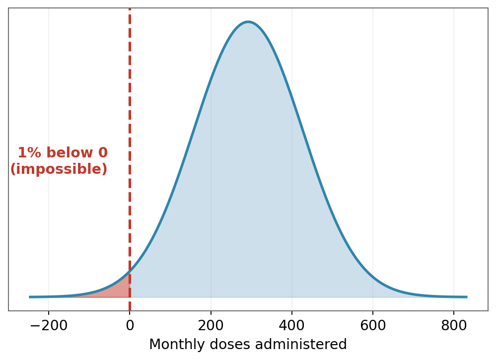
Lower bound

\[L = 0\]

A structural constraint. Monthly doses administered cannot be negative.

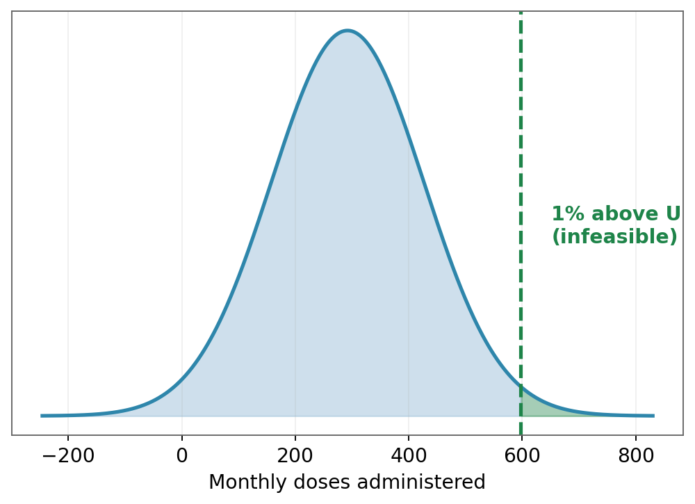
Upper bound

\[U_{i,v,t} = k_{i,v}\,E_{i,v,t}, \quad E_{i,v,t} = \tfrac{P_{i,v,y}\,\tau_{v,y}\,d_v}{12}\]

FSP expected monthly doses \(E\) (\(P\) = target population, \(\tau\) = WHO coverage, \(d\) = doses per child), scaled by \(k_{i,v} = Q_{0.975}\!\left(\tfrac{y}{E}\,\big|\,\mathcal{C}\right)\) calibrated on 2018 to 2019.

From bounds to truncated distribution

Once \([L, U]\) is set, the raw Gaussian forecast is re-cast as a truncated Normal on that interval.

\[Y_{i,v,t+h} \sim \mathcal{N}(\mu, \sigma) \;\Longrightarrow\; Y_{i,v,t+h} \sim \mathrm{TN}(\mu, \sigma, L, U)\]

Standardised bounds and normaliser (\(\Phi\), \(\phi\): standard Normal CDF and PDF):

\[\alpha = \frac{L-\mu}{\sigma},\qquad \beta = \frac{U-\mu}{\sigma},\qquad Z = \Phi(\beta) - \Phi(\alpha)\]

Truncated mean and variance:

\[\mu^{\mathrm{tr}} = \mu + \sigma\,\frac{\phi(\alpha) - \phi(\beta)}{Z}, \qquad (\sigma^{\mathrm{tr}})^2 = \sigma^2\!\left[1 + \frac{\alpha\,\phi(\alpha) - \beta\,\phi(\beta)}{Z} - \left(\frac{\phi(\alpha)-\phi(\beta)}{Z}\right)^{2}\right]\]

The truncated distribution is scored with the exact closed-form truncated Normal CRPS.

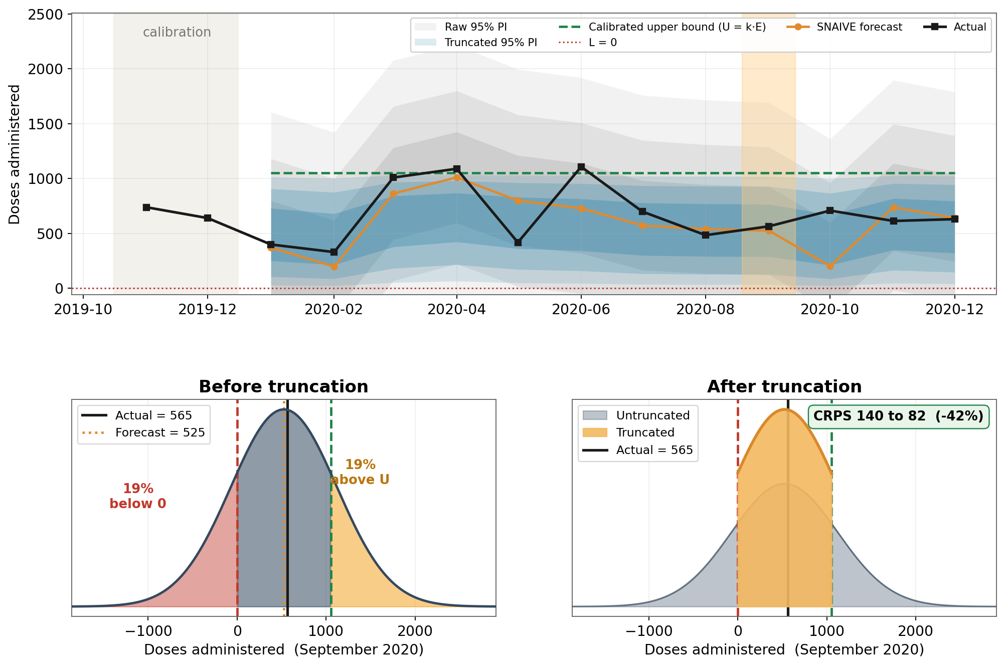
Truncation in practice

The untruncated raw Gaussian wastes mass below 0 and above \(U\). Truncation concentrates it into the feasible range, improving the CRPS.

Evaluation metrics

Errors are scaled by the FSP benchmark, so a value below 1 beats current practice.

Point accuracy

\[\mathrm{MSE} = \tfrac{1}{n}\sum_t (y_t-\hat{y}_t)^2 \qquad \mathrm{MAE} = \tfrac{1}{n}\sum_t |y_t-\hat{y}_t|\]

\[\mathrm{RMSSE} = \sqrt{\tfrac{\mathrm{MSE}}{\mathrm{MSE}_{\mathrm{FSP}}}} \qquad \mathrm{MASE} = \tfrac{\mathrm{MAE}}{\mathrm{MAE}_{\mathrm{FSP}}}\]

Pooled across series: \(\;\mathrm{RMSSE}_{\text{pooled}} = \sqrt{\tfrac{1}{N}\textstyle\sum_i \mathrm{RMSSE}_i^{2}}\)

Distributional accuracy

\[\mathrm{CRPS}(F,y) = \int_{-\infty}^{\infty}\big(F(x)-\mathbf{1}\{x\ge y\}\big)^2\,dx\]

\[\text{scaled CRPS} = \tfrac{\mathrm{CRPS}}{\mathrm{CRPS}_{\mathrm{FSP}}}\]

Truncated forecasts are scored with the closed-form CRPS of \(\mathrm{TN}(\mu,\sigma,0,U)\), not the raw Gaussian.

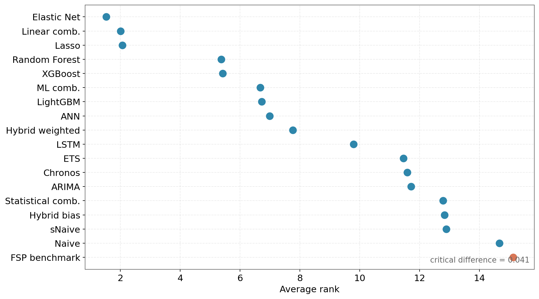
How to read the scale Below 1 beats the FSP tool, 1 ties, above 1 is worse. Ranking via the Nemenyi test, \(\mathrm{CD} = q_\alpha\sqrt{k(k+1)/6N}\); methods whose bars overlap are not significantly different.

Outline

• Background and motivation
• Current practice: the FSP tool
• Data and Methodology
• Results

Results: before truncation

Method	MASE	RMSSE	Scaled CRPS	Runtime (s)
Elastic Net	0.002	0.003	0.002	0.53
Linear comb.	0.002	0.003	0.003	1.09
Lasso	0.003	0.004	0.004	0.62
XGBoost	0.063	0.091	0.059	1.17
Random Forest	0.021	0.042	0.059	60.49
ML comb.	0.045	0.067	0.060	63.30
LightGBM	0.079	0.111	0.079	2.28
ANN	0.113	0.228	0.116	20.03
Hybrid weighted	0.204	0.370	0.182	4165.58
LSTM	0.292	0.654	0.271	25.18
ETS	0.417	0.689	0.348	4.18
Chronos	0.415	0.554	0.350	23.21
ARIMA	0.436	0.569	0.366	10.84
Statistical comb.	0.404	0.526	0.372	4134.03
Hybrid bias	0.420	0.481	0.412	4165.58
sNaive	0.510	0.666	0.433	2.07
Naive	0.591	0.776	0.575	2.01
FSP benchmark	1.000	1.000	1.000	0.87

Who wins before truncation

RMSSE (point accuracy)

Scaled CRPS (distribution)

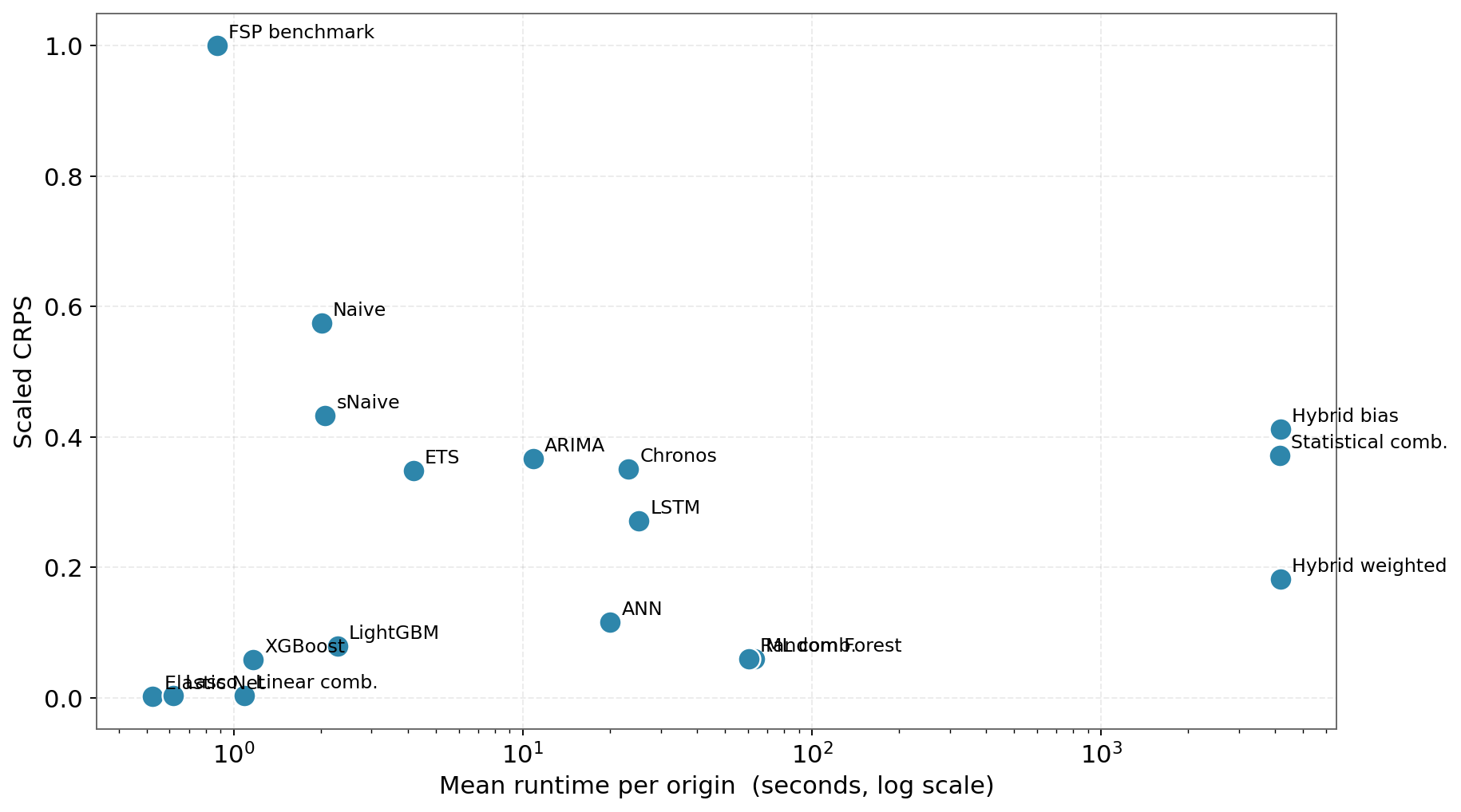
Accuracy vs computational cost

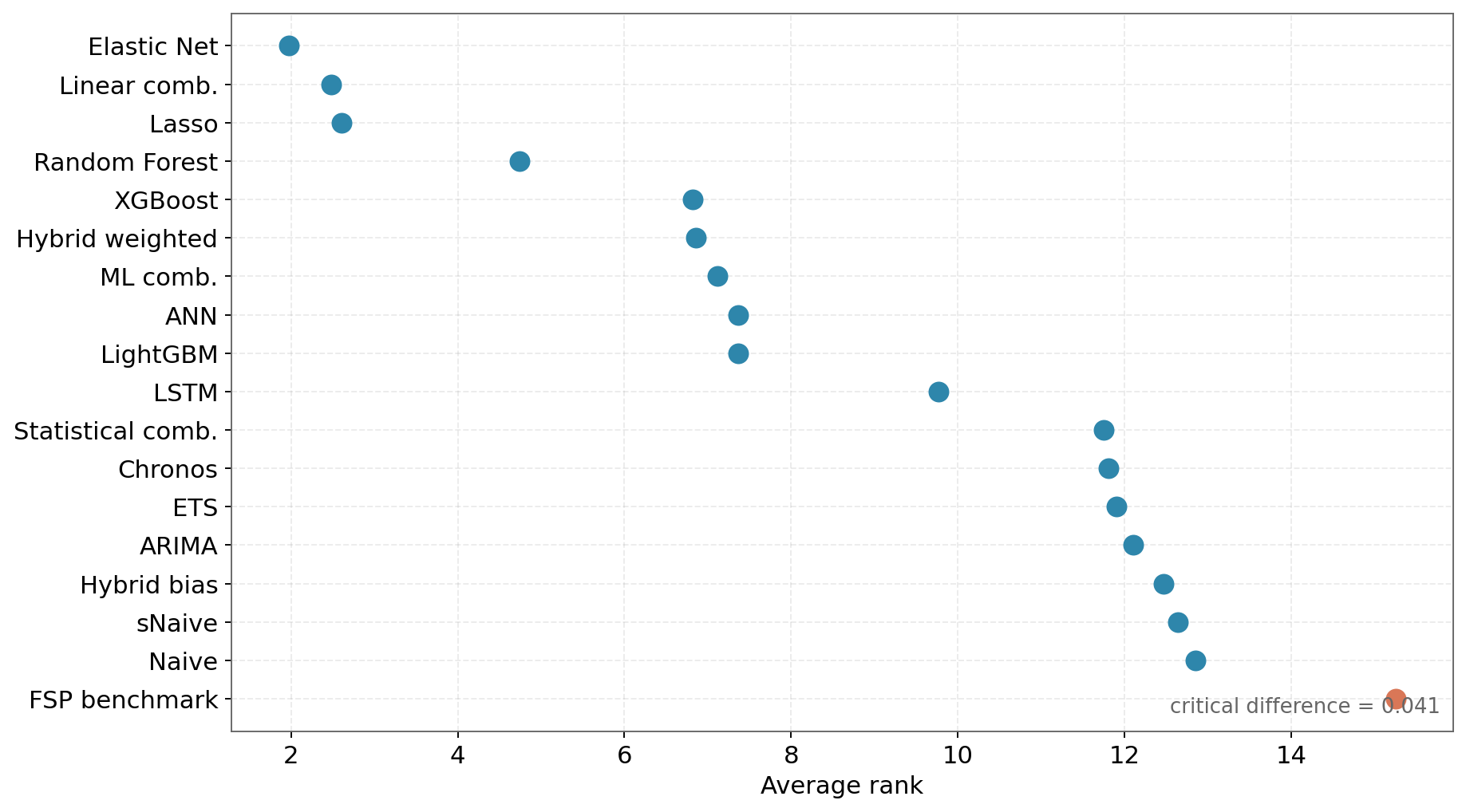
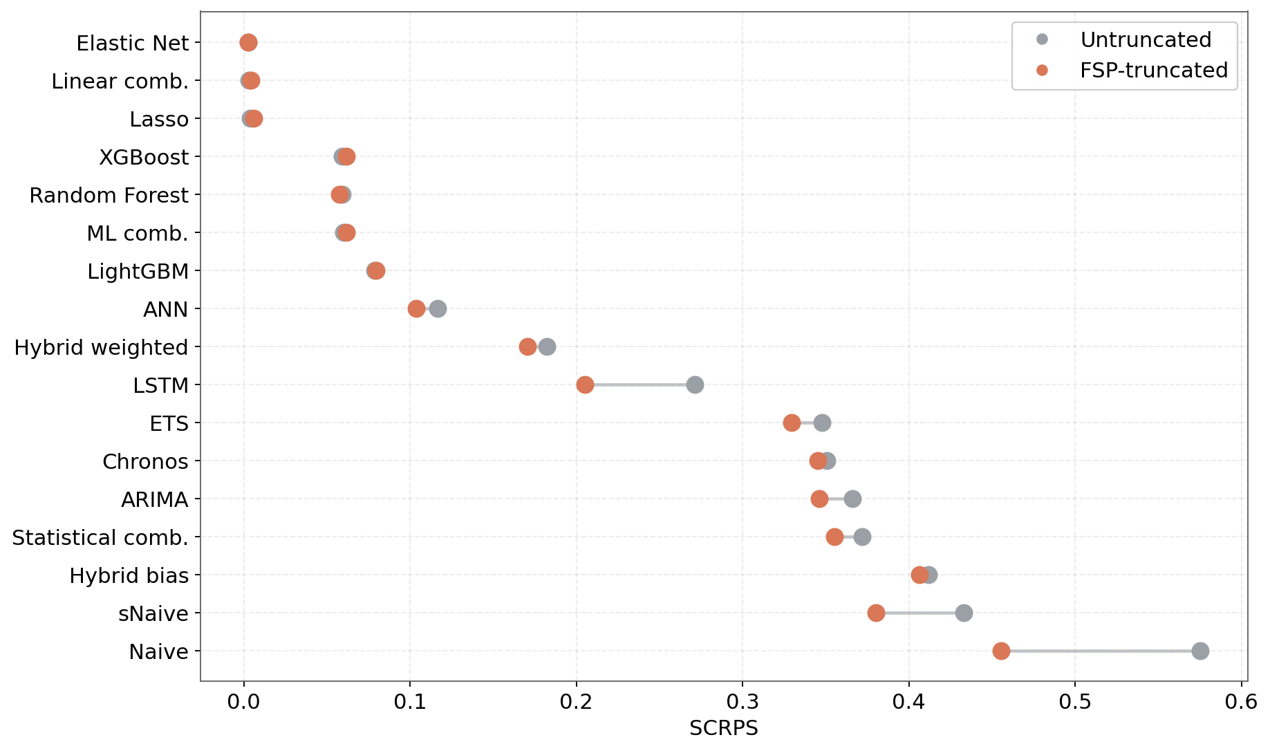
After truncation: scaled CRPS

Truncation moves every method to the left (better). Gains are largest for the most diffuse forecasters, such as LSTM, sNaive and ETS.

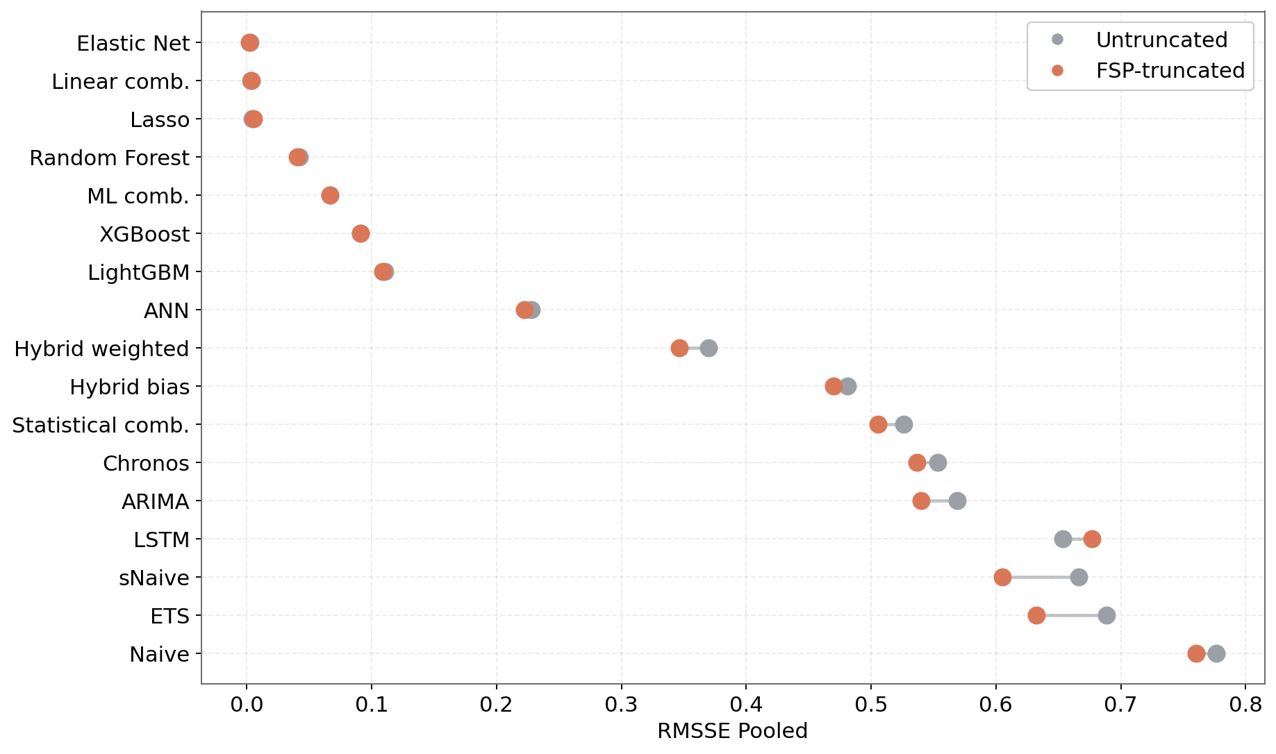
After truncation: RMSSE

The road ahead

Where this work goes next.

Add the wastage component

• Extend administered forecasts to total consumption
• Supports end-to-end procurement quantification

Link to inventory simulation

• Translate forecast distributions into stockouts, wastage, and service levels

Hierarchical reconciliation

• Keep forecasts coherent across national → sub-county levels

Any questions or thoughts? 💬

Visit my website for slides