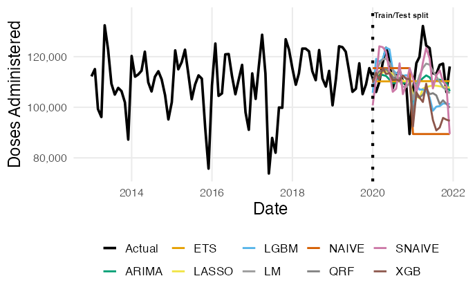
| Model class | Models |
|---|---|
| Classical statistical | ETS, ARIMA, Naïve, Seasonal Naïve |
| Regression-based | Linear regression, LASSO |
| Machine learning | Quantile Random Forest, XGBoost, LightGBM |

Distributional Post-Processing for Vaccine Demand Inventory Forecasting
Udeshi Salgado, DL4SG, Cardiff University, UK
Lead Supervisor: Professor Bahman Rostami-Tabar
Co-supervisors: Dr Thanos E Goltsos, Dr Geraint Palmer, Dr Xun Wang
13 March 2026
Background
1 in 5 children worldwide still lack access to essential vaccines.
A key operational contributor is inefficiency in vaccine supply chains.
In low- and middle-income countries, these inefficiencies often involve:
- inaccurate demand forecasts
- inventory decisions made under limited uncertainty information
- wastage and stockouts
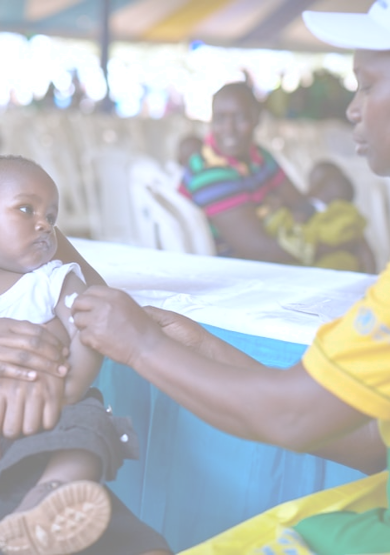
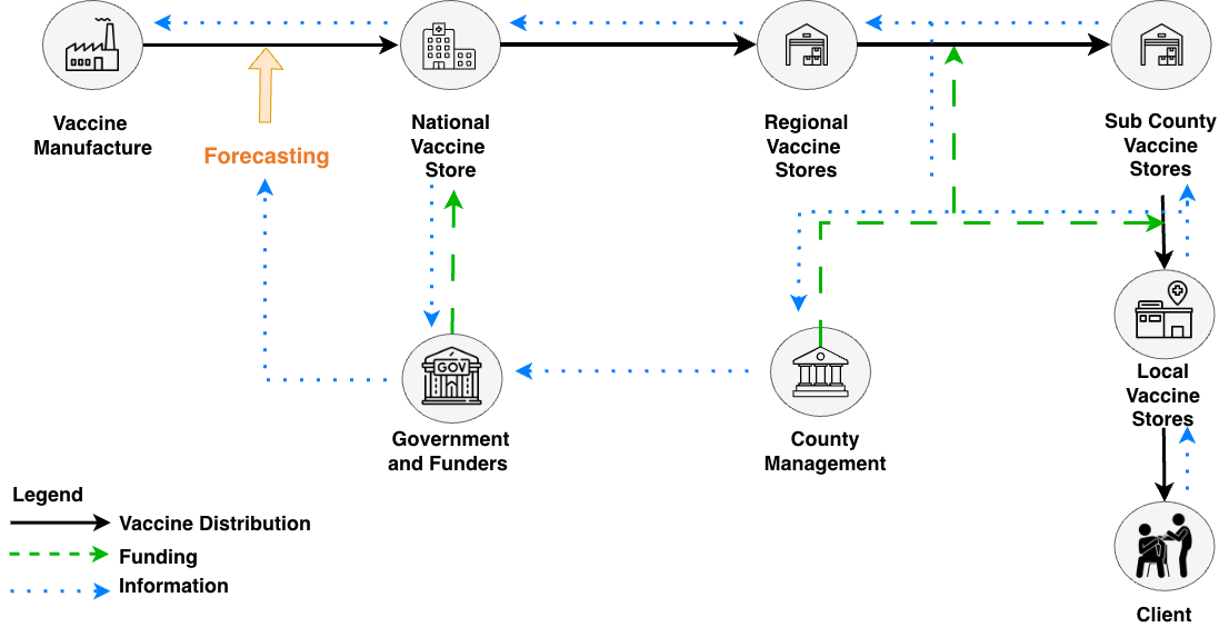
The Immunisation Supply Chain
BCG (Bacille Calmette-Guérin) Vaccines

Vial

Dose

Administered
The Problem: Evidence from the Study Setting
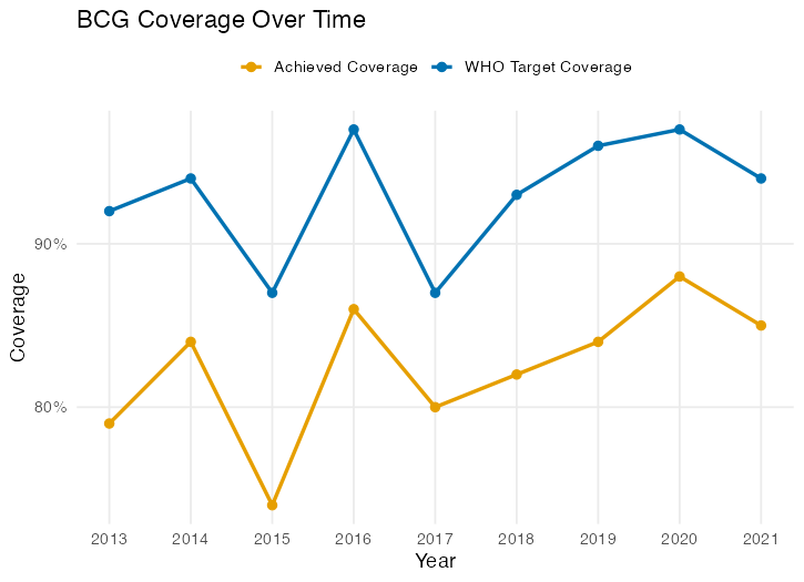
- Coverage shown here refers to BCG vaccination coverage among newborns
- BCG is a single-dose vaccine administered at birth
- Coverage is defined as:
\[ \text{Coverage} = \frac{\text{No of Clients Administered}}{\text{Target Population}} \]
- Forecasting limitations may contribute to persistent coverage gaps.
The FSP Forecasting
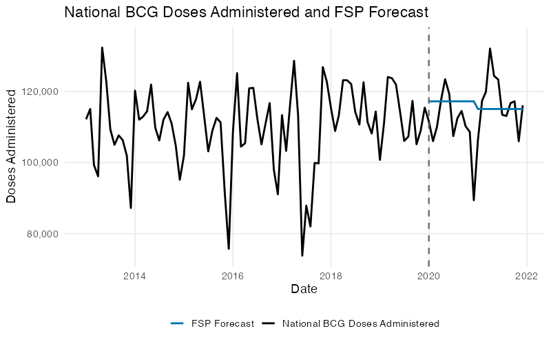
Forecast equation for doses administered:
\[ \hat{D_t} = \frac{P_y \cdot C_y}{12} \]
Where:
- \(\hat{D_t}\): Forecasted doses administered at month \(t\)
- \(P_t\): Target population at year \(y\)
- \(C_t\): WHO target coverage at year \(y\)
The Risk of Point Forecasting
Addressing the Uncertainty
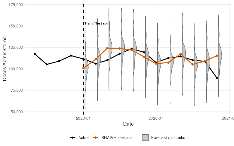
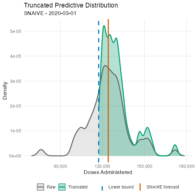
Distributional Post-Processing: Defining Lower Bound
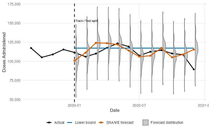
We define lower bound as the FSP forecast:
\[ \text{Lower Bound} = \frac{P_y \cdot C_y}{12} \]
Where:
- \(P_t\): Target population at year \(y\)
- \(C_t\): WHO target coverage at year \(y\)
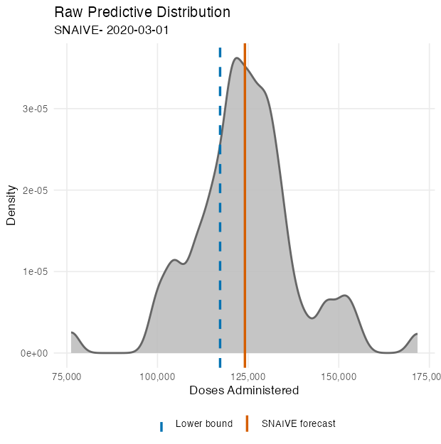
Distributional Post-Processing: Truncation
Connect
Udeshi Salgado
2nd year PhD Student
DL4SG, Cardiff University, UK
LinkedIn: udeshi-salgado
Slides:

Outline of my talk
- Problem Statement and Motivation
- Decision-Relevant Forecasting under Uncertainty
- Forecasting Framework
- Distributional Post-Processing and Inventory Decision Model
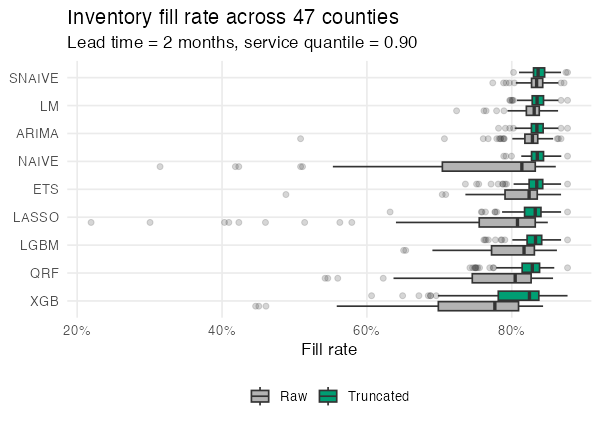
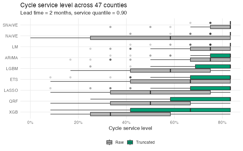
- Results